Code
print("We have " + str(len(data)) + " total different movies and TV shows that we are working with.")We have 4985 total different movies and TV shows that we are working with.The present article analyzes a dataset containing information about titles on different streaming services and build a model to predict the popularity of an arbitrary title. The datasets used were sourced from Kaggle and the specific links can be found on the Data tab above. These provide valuable insights into the popularity and characteristics of different titles available on the streaming platforms and will help us in predicting the outcomes of future titles.
The streaming services industry has seen rapid growth in recent years and has undoubtedly revolutionized the way we consume content. With numerous platforms offering a vast array of media types, it has become increasingly important for creators and streaming platforms to understand what makes a certain movie or TV show popular. This project aims to explore the Kaggle dataset and uncover the key factors that contribute to their popularity through fitting a series of different models.
We developed a web app that predicts a score for a show or movie given particular inputs. The hope is to give producers an idea of how popular a show or movie will be before they spend the time and money on producing it. This analysis is important because it shows how data can be used to create media people actaully want.
We have a column in our dataset description that describes each show and movie. I think it would have been interesting to use word vectoriztion and natural language processing (NLP) to quantify this. If we were to expand on this project, adding an NLP component would be one avenue to do so. A neural network may have also been an interesting model to apply. Neural networks are considered to be highly flexible but not very interpretable, so adding this model to the app may or may not have been beneficial. In a practical sense, the model should be somewhat interpretable if order to use with the web app, however, predictive power is beneficial in its own right.
We combined the below four datasets found on Kaggle to get a comprehensive dataset of movies and TV shows available on the major streaming platforms.
The dataset contains both categorical and numeric variables which may provide insights for our analysis. Here is a brief description of the key variables:
type: Indicates whether the show is a TV series or a movie.title: The title of the TV show.director: The name of the director(s) of the show.cast: The names of the main cast members.country: The countries the show was released in.release_year: The year when the show was released.rating: The content rating assigned to the show (TV-14, PG-13, etc.).duration: The number of seasons (for TV series) or the duration (minutes) of the movie (for movies).listed_in: The genre(s) or category(s) the show belongs to.description: A brief summary or description of the show.score: Rating of the show or movie - scraped from IMDb.director_score: Calculated score based on the directors of the title.Together, these variables provide a set of features that allow us to analyze and understand the characteristics that determine the popularity of TV shows. By exploring these variables and their relationships, we can gain insights into the factors that contribute to a show’s popularity, like the impact of different genres or countries of origin, and begin to create better shows that more people would watch.
Due to the four original datasets being from Kaggle and in the same format we were able to merge them into one dataset that encompassed all of the previously mentioned streaming sites. The main area of concern with this dataset were the missing IMDb scores as that is the key metric we were using for our modeling. Another concern is that directors and casts members were in lists and this will prove to be difficult to feed to our model.
To fill in the missing IMDb scores we used an API that can be found here. In order to use the API we made a python script using the requests library that would query the API with the title of the show or movie we wanted the score for. From there the API searches its internal database and would pull the IMDb score from there. From there our python script would append our dataset with the score pulled from the API.
Since we wanted to use each director and cast member as their own predictor we had to get the overall average IMDb score for each director or cast member. A challenge we overcame was that each row stored their cast members or directors as a list. This would make it hard to compute the average since we would not be able to iterate over each cast member or director this way. In order to solve this, we split the lists and make each director or cast member their own respective row. From here we were able to iterate over each cast member or director and compute their average score. Computing the average score bring into question data leakage because some values from the response would be used to make predictors. To prevent this from happening, we split the entire dataset in half, and computed the averages on only one half of the dataset. We used the other half of the dataset, now imputed with the average scores, for training and testing. After the averages were computed for the directors and cast members the train dataset and test were merged back together to be fed into the models.
For Genre we had some values that had multiple alliases such as Not Rated and NR being the same value but when we use our one-hot encoding to vectorize these for use as predictors it would read them as seperate values. In order to prevent this we had to come up with a normalized naming scheme. In order to normalize the naming scheme we searched for unique genre values and merged all common values into a uniform name so that they can now be one-hot encoded.
The response varaible that we used for prediction was the IMDb score of the Movie or TV Show. After combing the four datasets we found on Kaggle we discovered some of the shows had null values for their IMDb score. In order to replace these nulls we connected to an API that can be found here. With this API we were able to query by Movie or Show Title and get it’s IMDb score. We then cleaned and formatted our data so that it could be vectorized for our models. Since cast, director, and country of origin were all in lists, we had to split each list value into their own rows. Due to this spliting we can turn our categorical variables into numerical representation in order for our model to read it.
In this section we will explore and visualize our dataset to gain a better understanding of what we are working with, identify any obvious patterns, correlations, or trends.
print("We have " + str(len(data)) + " total different movies and TV shows that we are working with.")We have 4985 total different movies and TV shows that we are working with.print(data.shape)
print("There are a total of 89 columns that were are working with.")(4985, 89)
There are a total of 89 columns that were are working with.import seaborn as sns
sns.countplot(x=data["type"])
# Add labels and title
plt.xlabel("Type")
plt.ylabel("Count")
plt.title("Distribution of Titles by Type")
# Display the plot
plt.show()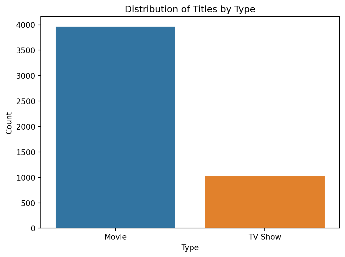
# 1. Line Chart of the Number of Titles Released per Year

# Group data by year and count number of titles
counts = data.groupby("release_year")["title"].count()

# Create line chart
#plt.figure(figsize=(10,10))
plt.plot(counts.index, counts.values)

# Add labels and title
plt.xlabel("Year")
plt.ylabel("Number of Titles Released")
plt.title("Number of Titles Released per Year")

# Display chart
plt.show()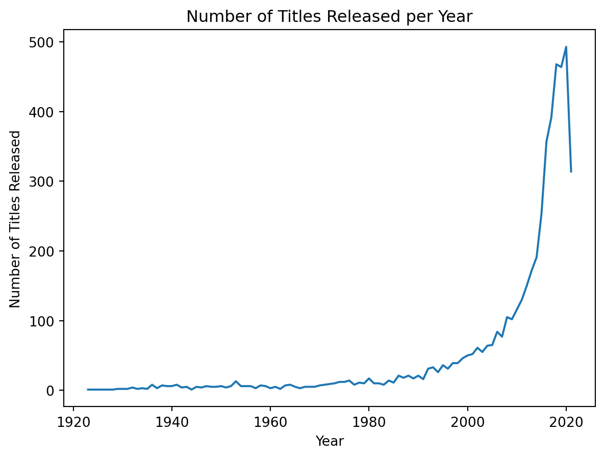
# 2. Histogram of the Distribution of Content Ratings

# Create histogram of content ratings
#plt.figure(figsize=(20,10))
plt.hist(data["rating"].dropna(), bins=10)

# Add labels and title
plt.xlabel("Content Rating")
plt.xticks(rotation=45)
plt.ylabel("Frequency")
plt.title("Distribution of Content Ratings")

# Display chart
plt.show()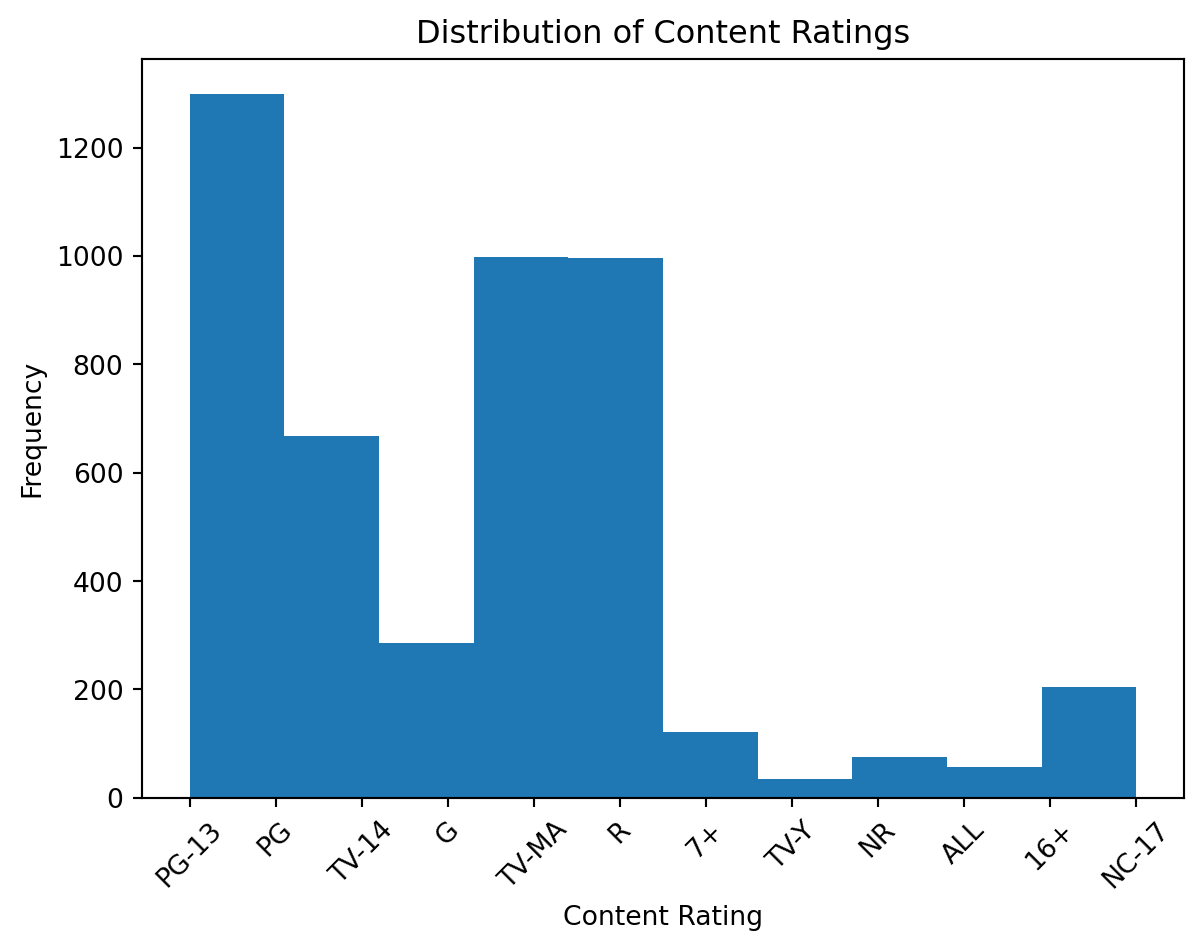
# 3. Bar Chart of the Number of Titles per Country (count > 10)

# Extract first country from country column
chart = data.copy()
chart["country"] = chart["country"].str.split(", ").str[0]

# Group data by country and count number of titles
counts = chart.groupby("country")["title"].count()
counts = counts[counts > 10].sort_values(ascending=False)

# Create bar chart
#plt.figure(figsize=(20,10))
plt.bar(counts.index, counts.values)

# Add labels and title
plt.xlabel("Country")
plt.xticks(rotation=90)
plt.ylabel("Number of Titles")
plt.title("Number of Titles per Country")

# Display chart
plt.show()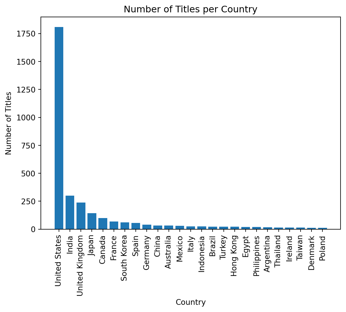
# 4. Movie and Rating Scatter Plot

# Filter out TV shows and missing ratings
movies = data[(data["type"] == "Movie") & (data["score"].notnull())]

# Create scatter plot of IMDb rating vs. runtime
#plt.figure(figsize=(20,10))
plt.scatter(movies["score"], movies["duration"], alpha=0.5)

# Add labels and title
plt.xlabel("IMDb Rating")
plt.ylabel("Runtime (minutes)")
plt.title("IMDb Rating vs. Runtime for Movies")

# Display chart
plt.show()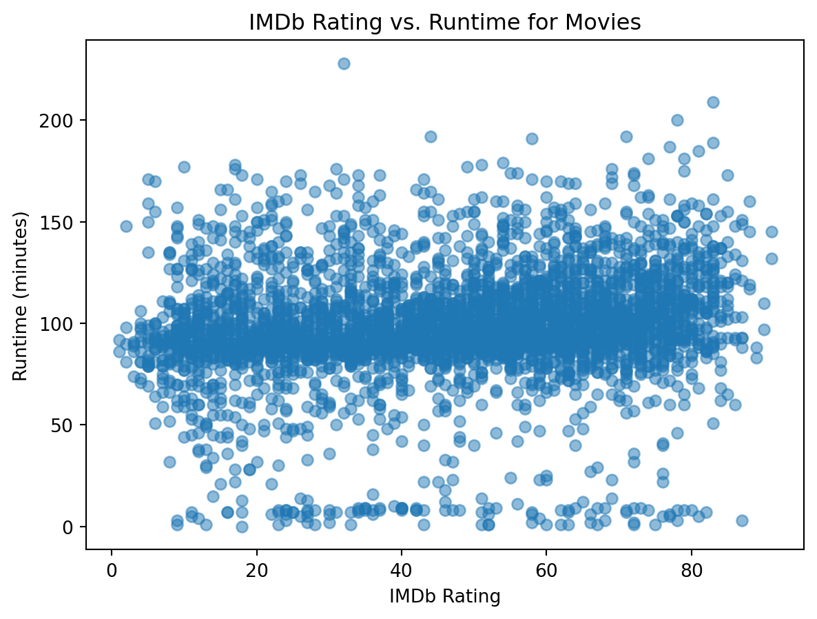
# 5. TV Show and Rating Scatter Plot

# Filter out Movies and missing ratings
tv = data[(data["type"] == "TV Show") & (data["score"].notnull())]

# Create scatter plot of IMDb rating vs. runtime
#plt.figure(figsize=(20,10))
plt.scatter(tv["score"], tv["duration"], alpha=0.5)

# Add labels and title
plt.xlabel("IMDb Rating")
plt.ylabel("Runtime (seasons)")
plt.title("IMDb Rating vs. Runtime for TV Shows")

# Display chart
plt.show()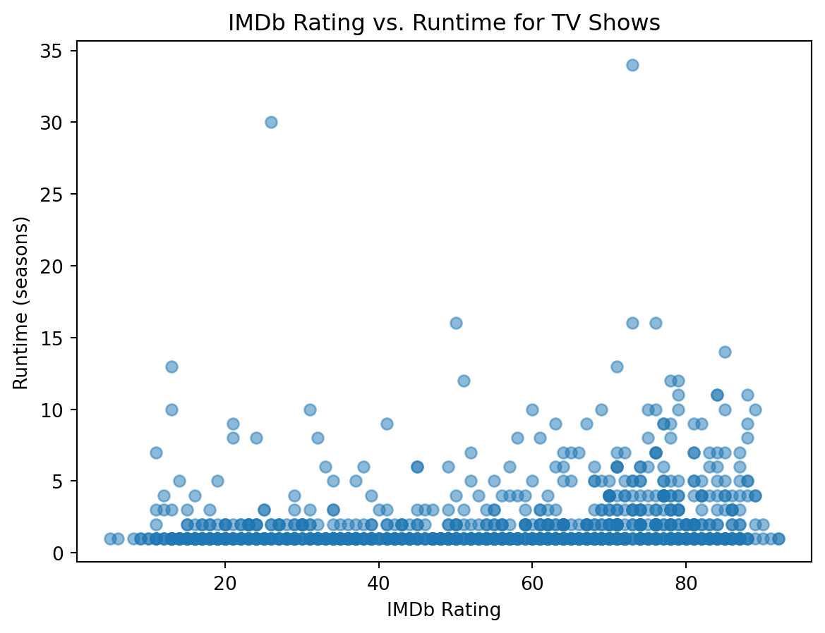
# 6. Top 15 Genres By Number of Titles

# Get list of genre columns
genre_cols = [col for col in data.columns if col.startswith("genre")]

# Sum the number of true values in each genre column to get the total number of titles for each genre
genre_counts = data[genre_cols].sum()#.sort_values(ascending=False)

# Get the top 10 genres by number of titles
top_genres = genre_counts[:15]

# Remove "genre." from the genre names in the x-axis labels
labels = [col.replace("genre.", "") for col in top_genres.index]

# Create bar chart
# plt.figure(figsize=(20, 10))
plt.bar(labels, top_genres.values, color='purple')

# Add labels and title
plt.xlabel("Genre")
plt.xticks(rotation=45, ha='right')
plt.ylabel("Number of Titles")
plt.title("Top 10 Genres by Number of Titles")

# Display chart
plt.show()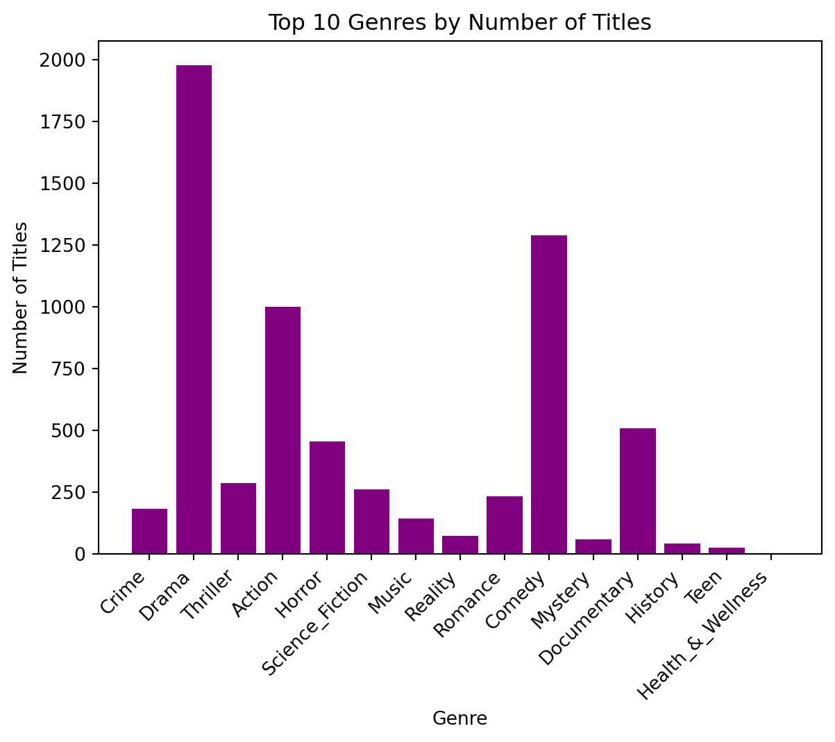
These visualizations revealed several intriguing patterns. We almost have an 80/20 split of movies and shows within our data. The number of released titles per year is exponential, and is only hindered in 2020, due to the COVID-19 pandemic limiting production. The few bar plots also demonstrate the ratings, major countries, and the types of media within the dataset. Now we have a much better picture of the data that we are working with and can keep this in mind for our future models.
In this section, we describe the machine learning models employed for predicting the popularity score of TV shows and movies in our project. We utilized several models, including beta regression, decision tree, K-Nearest Neighbors (KNN), and random forest. Each of these models offers unique characteristics and can capture different aspects of the data to make accurate predictions.
To evaluate the performance of our machine learning models, we employed a train-test split approach. This process involves dividing our dataset, consisting of TV shows and movies, into two separate subsets: a training set and a testing set. The training set, which constitutes a majority of the data, was used to train our models to learn the underlying patterns and relationships between the features and the target variable, which in our case is the popularity score. The testing set, on the other hand, served as an unseen dataset to assess the models’ generalization ability and determine their predictive performance on new, unseen instances. By randomly assigning the data points to the training and testing sets, we ensured that the evaluation process is unbiased and representative of real-world scenarios. After fitting each model with the training set, we are left with the root mean squared error (rMSE) value.
This metric gives us the weighted distance our model is from the correct metric. We found that the response variable score has a sample standard deviation of 21.7. This means that if we guessed the mean every time, we would be, on average, off by 21.7 points. So, our model should try to minimize the rMSE and get at most a rMSE of 21.7.
For all of these models, we defined the set of predictor variables to be the same. These predictors included genre information, duration, release year, type, rating, director’s average score, cast’s average score, and country.
Also, to evaluate all four model’s performance and validate its predictive ability, we employed a cross-validation strategy. Code was written so that the dataset was divided into five subsets or folds, with each fold serving as a testing set while the remaining four folds were used for training. The grid search was performed within this cross-validation framework, optimizing the model’s hyperparameters based on the negative root mean squared error (RMSE) metric. By utilizing cross-validation, we obtained robust estimates of the model’s performance and ensured the generalization of the results to unseen data.
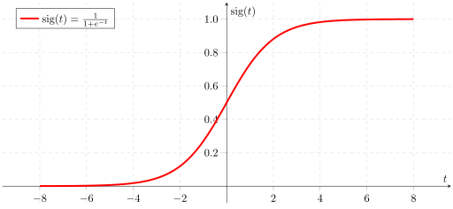
Beta regression is a statistical model specifically designed for modeling continuous variables bounded between 0 and 1. In our case, we used beta regression to predict the popularity score, which ranges from 0 to 100. Beta regression takes into account the distributional characteristics of the data and can handle the inherent boundedness of the popularity score, allowing for accurate predictions. It uses an underlying logistic function to transform a linear regression.
We decided to fit a beta regression as opposed to a linear regression because we wanted the model to predict values only within the range [0,100]. A beta regression allows us to specify this range.
Our pipeline was structured as follows:
Pipeline(steps=[('predictors',
                 ColumnSelector(columns=['genre.Crime', 'genre.Drama',
                                         'genre.Thriller', 'genre.Action',
                                         'genre.Horror',
                                         'genre.Science_Fiction', 'genre.Music',
                                         'genre.Reality', 'genre.Romance',
                                         'genre.Comedy', 'genre.Mystery',
                                         'genre.Documentary', 'genre.History',
                                         'genre.Teen',
                                         'genre.Health_&_Wellness',
                                         'genre.Lifestyle', 'genre.Culture',
                                         'genre.Blac...
                                         'genre.LGBTQ', 'genre.Adult_Animation',
                                         'genre.Sitcom', ...])),
                ('columntransform',
                 ColumnTransformer(remainder='passthrough',
                                   transformers=[('numericnaonehotencoder',
                                                  NumericNAOneHotEncoder(),
                                                  <sklearn.compose._column_transformer.make_column_selector object at 0x12d6d6520>),
                                                 ('onehotencoder',
                                                  OneHotEncoder(),
                                                  ['type', 'rating',
                                                   'country'])])),
                ('beta', BetaRegression(from_range=(0, 100)))])
In a Jupyter environment, please rerun this cell to show the HTML representation or trust the notebook. Pipeline(steps=[('predictors',
ColumnSelector(columns=['genre.Crime', 'genre.Drama',
'genre.Thriller', 'genre.Action',
'genre.Horror',
'genre.Science_Fiction', 'genre.Music',
'genre.Reality', 'genre.Romance',
'genre.Comedy', 'genre.Mystery',
'genre.Documentary', 'genre.History',
'genre.Teen',
'genre.Health_&_Wellness',
'genre.Lifestyle', 'genre.Culture',
'genre.Blac...
'genre.LGBTQ', 'genre.Adult_Animation',
'genre.Sitcom', ...])),
('columntransform',
ColumnTransformer(remainder='passthrough',
transformers=[('numericnaonehotencoder',
NumericNAOneHotEncoder(),
<sklearn.compose._column_transformer.make_column_selector object at 0x12d6d6520>),
('onehotencoder',
OneHotEncoder(),
['type', 'rating',
'country'])])),
('beta', BetaRegression(from_range=(0, 100)))])ColumnSelector(columns=['genre.Crime', 'genre.Drama', 'genre.Thriller',
'genre.Action', 'genre.Horror', 'genre.Science_Fiction',
'genre.Music', 'genre.Reality', 'genre.Romance',
'genre.Comedy', 'genre.Mystery', 'genre.Documentary',
'genre.History', 'genre.Teen',
'genre.Health_&_Wellness', 'genre.Lifestyle',
'genre.Culture', 'genre.Black_Stories', 'genre.News',
'genre.Latino', 'genre.Adventure', 'genre.Anime',
'genre.Talk_Show', 'genre.Sketch_Comedy',
'genre.Family', 'genre.Kids', 'genre.Classics',
'genre.LGBTQ', 'genre.Adult_Animation', 'genre.Sitcom', ...])ColumnTransformer(remainder='passthrough',
transformers=[('numericnaonehotencoder',
NumericNAOneHotEncoder(),
<sklearn.compose._column_transformer.make_column_selector object at 0x12d6d6520>),
('onehotencoder', OneHotEncoder(),
['type', 'rating', 'country'])])<sklearn.compose._column_transformer.make_column_selector object at 0x12d6d6520>
NumericNAOneHotEncoder()
['type', 'rating', 'country']
OneHotEncoder()
['genre.Crime', 'genre.Drama', 'genre.Thriller', 'genre.Action', 'genre.Horror', 'genre.Science_Fiction', 'genre.Music', 'genre.Reality', 'genre.Romance', 'genre.Comedy', 'genre.Mystery', 'genre.Documentary', 'genre.History', 'genre.Teen', 'genre.Health_&_Wellness', 'genre.Lifestyle', 'genre.Culture', 'genre.Black_Stories', 'genre.News', 'genre.Latino', 'genre.Adventure', 'genre.Anime', 'genre.Talk_Show', 'genre.Sketch_Comedy', 'genre.Family', 'genre.Kids', 'genre.Classics', 'genre.LGBTQ', 'genre.Adult_Animation', 'genre.Sitcom', 'genre.Cooking_&_Food', 'genre.Sports', 'genre.Game_Shows', 'genre.International', 'genre.Cartoons', 'genre.Science_&_Technology', 'genre.Stand_Up', 'genre.Special_Interest', 'genre.Suspense', 'genre.TV_Shows', 'genre.Arts,_Entertainment,_and_Culture', 'genre.Variety', 'genre.Fantasy', 'genre.Young_Adult_Audience', 'genre.Animation', 'genre.Western', 'genre.Arthouse', 'genre.Unscripted', 'genre.Faith_and_Spirituality', 'genre.Military_and_War', 'genre.Independent_Movies', 'genre.British_TV_Shows', 'genre.Romantic_Movies', 'genre.Musical', 'genre.Comedies', 'genre.Classic_Movies', "genre.Kids'_TV", 'genre.Nature', 'genre.Cult', 'genre.Korean_TV_Shows', 'genre.Movies', 'genre.Biographical', 'genre.Superhero', 'genre.Coming_of_Age', 'genre.Anthology', 'genre.Buddy', 'genre.Parody', 'genre.Spy/Espionage', 'genre.Survival', 'genre.Soap_Opera_/_Melodrama', 'genre.Dance', 'genre.Medical', 'genre.Disaster']
passthrough
BetaRegression(from_range=(0, 100))
First, we selected the predictors we wanted to use. Then, we one hot encoded the categorical variables. Simultaneously, we dealt with missing numerical values by encoding if a value was missing and filling it with a 0 if it was. We add our model as the last step in the pipeline.
The best cross-evaluation score for this model was a root mean squared error of 19.26. We can loosely interpret this as saying our model is, on average, 19.26 IMDb rating points off from the actual score.
The beta regression achieved a test rMSE of 19.71. This is about a 2 point difference from the sample standard deviation of the scores (21.7), which means the beta regression predicts about 2 rating points more accurately than guessing the mean, on average.
K-Nearest Neighbors is a non-parametric algorithm that makes predictions based on the similarity of a given data point to its k nearest neighbors in the feature space. In our case, KNN is used to predict the popularity score by finding the k most similar instances in the training data. KNN would be particularly suitable if similar shows or movies tend to have similar scores.
Our pipeline was structured as follows:
Pipeline(steps=[('predictors',
                 ColumnSelector(columns=['genre.Crime', 'genre.Drama',
                                         'genre.Thriller', 'genre.Action',
                                         'genre.Horror',
                                         'genre.Science_Fiction', 'genre.Music',
                                         'genre.Reality', 'genre.Romance',
                                         'genre.Comedy', 'genre.Mystery',
                                         'genre.Documentary', 'genre.History',
                                         'genre.Teen',
                                         'genre.Health_&_Wellness',
                                         'genre.Lifestyle', 'genre.Culture',
                                         'genre.Blac...
                 ColumnTransformer(remainder='passthrough',
                                   transformers=[('numericnaonehotencoder',
                                                  NumericNAOneHotEncoder(),
                                                  <sklearn.compose._column_transformer.make_column_selector object at 0x12d6b0d00>),
                                                 ('onehotencoder',
                                                  OneHotEncoder(),
                                                  ['type', 'rating',
                                                   'country'])])),
                ('knn',
                 TransformedTargetRegressor(regressor=KNeighborsRegressor(n_neighbors=17,
                                                                          weights='distance')))])
In a Jupyter environment, please rerun this cell to show the HTML representation or trust the notebook. Pipeline(steps=[('predictors',
ColumnSelector(columns=['genre.Crime', 'genre.Drama',
'genre.Thriller', 'genre.Action',
'genre.Horror',
'genre.Science_Fiction', 'genre.Music',
'genre.Reality', 'genre.Romance',
'genre.Comedy', 'genre.Mystery',
'genre.Documentary', 'genre.History',
'genre.Teen',
'genre.Health_&_Wellness',
'genre.Lifestyle', 'genre.Culture',
'genre.Blac...
ColumnTransformer(remainder='passthrough',
transformers=[('numericnaonehotencoder',
NumericNAOneHotEncoder(),
<sklearn.compose._column_transformer.make_column_selector object at 0x12d6b0d00>),
('onehotencoder',
OneHotEncoder(),
['type', 'rating',
'country'])])),
('knn',
TransformedTargetRegressor(regressor=KNeighborsRegressor(n_neighbors=17,
weights='distance')))])ColumnSelector(columns=['genre.Crime', 'genre.Drama', 'genre.Thriller',
'genre.Action', 'genre.Horror', 'genre.Science_Fiction',
'genre.Music', 'genre.Reality', 'genre.Romance',
'genre.Comedy', 'genre.Mystery', 'genre.Documentary',
'genre.History', 'genre.Teen',
'genre.Health_&_Wellness', 'genre.Lifestyle',
'genre.Culture', 'genre.Black_Stories', 'genre.News',
'genre.Latino', 'genre.Adventure', 'genre.Anime',
'genre.Talk_Show', 'genre.Sketch_Comedy',
'genre.Family', 'genre.Kids', 'genre.Classics',
'genre.LGBTQ', 'genre.Adult_Animation', 'genre.Sitcom', ...])ColumnTransformer(remainder='passthrough',
transformers=[('numericnaonehotencoder',
NumericNAOneHotEncoder(),
<sklearn.compose._column_transformer.make_column_selector object at 0x12d6b0d00>),
('onehotencoder', OneHotEncoder(),
['type', 'rating', 'country'])])<sklearn.compose._column_transformer.make_column_selector object at 0x12d6b0d00>
NumericNAOneHotEncoder()
['type', 'rating', 'country']
OneHotEncoder()
['genre.Crime', 'genre.Drama', 'genre.Thriller', 'genre.Action', 'genre.Horror', 'genre.Science_Fiction', 'genre.Music', 'genre.Reality', 'genre.Romance', 'genre.Comedy', 'genre.Mystery', 'genre.Documentary', 'genre.History', 'genre.Teen', 'genre.Health_&_Wellness', 'genre.Lifestyle', 'genre.Culture', 'genre.Black_Stories', 'genre.News', 'genre.Latino', 'genre.Adventure', 'genre.Anime', 'genre.Talk_Show', 'genre.Sketch_Comedy', 'genre.Family', 'genre.Kids', 'genre.Classics', 'genre.LGBTQ', 'genre.Adult_Animation', 'genre.Sitcom', 'genre.Cooking_&_Food', 'genre.Sports', 'genre.Game_Shows', 'genre.International', 'genre.Cartoons', 'genre.Science_&_Technology', 'genre.Stand_Up', 'genre.Special_Interest', 'genre.Suspense', 'genre.TV_Shows', 'genre.Arts,_Entertainment,_and_Culture', 'genre.Variety', 'genre.Fantasy', 'genre.Young_Adult_Audience', 'genre.Animation', 'genre.Western', 'genre.Arthouse', 'genre.Unscripted', 'genre.Faith_and_Spirituality', 'genre.Military_and_War', 'genre.Independent_Movies', 'genre.British_TV_Shows', 'genre.Romantic_Movies', 'genre.Musical', 'genre.Comedies', 'genre.Classic_Movies', "genre.Kids'_TV", 'genre.Nature', 'genre.Cult', 'genre.Korean_TV_Shows', 'genre.Movies', 'genre.Biographical', 'genre.Superhero', 'genre.Coming_of_Age', 'genre.Anthology', 'genre.Buddy', 'genre.Parody', 'genre.Spy/Espionage', 'genre.Survival', 'genre.Soap_Opera_/_Melodrama', 'genre.Dance', 'genre.Medical', 'genre.Disaster']
passthrough
TransformedTargetRegressor(regressor=KNeighborsRegressor(n_neighbors=17,
weights='distance'))KNeighborsRegressor(n_neighbors=17, weights='distance')
KNeighborsRegressor(n_neighbors=17, weights='distance')
This is the same pipeline as in the beta regression, with the model swapped out for KNN.
For KNN, we tuned two hyperparameters: n_neighbors and weights. n_neighbors controls the number of nearest neighbors to be used when making a prediction. weights controls how the points are averaged to make that prediction: uniformly or by distance. We found that the best value for n_neighbors was 17, and the best method for weights was by weighting by distance. The highest cross evaluation score for KNN was a root mean squared error of 20.48.
The K-Nearest Neighbors model achieved a test rMSE of 20.52. This is about a 1 point difference from the sample standard deviation of the scores (21.7), which means the beta regression predicts about 1 rating point more accurately than guessing the mean, on average.
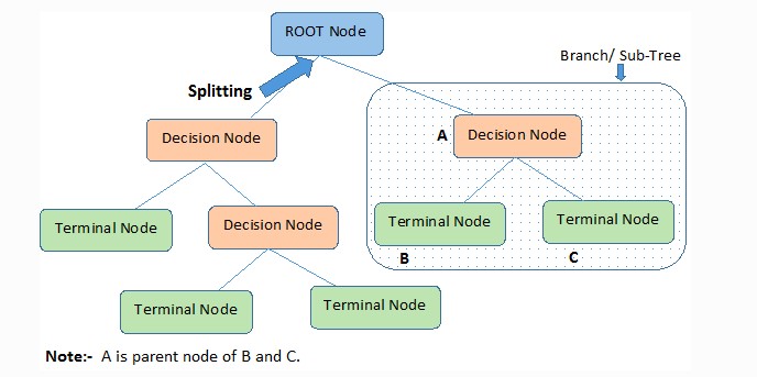
Decision trees are intuitive models that create a flowchart-like structure of decisions and their potential consequences. Each internal node represents a decision based on a specific feature, and each leaf node represents the predicted outcome (popularity score). Decision trees are capable of handling both numerical and categorical features, and they offer interpretability by visualizing the decision-making process.
Our pipeline is structured in the same way as our other models:
Pipeline(steps=[('predictors',
                 ColumnSelector(columns=['genre.Crime', 'genre.Drama',
                                         'genre.Thriller', 'genre.Action',
                                         'genre.Horror',
                                         'genre.Science_Fiction', 'genre.Music',
                                         'genre.Reality', 'genre.Romance',
                                         'genre.Comedy', 'genre.Mystery',
                                         'genre.Documentary', 'genre.History',
                                         'genre.Teen',
                                         'genre.Health_&_Wellness',
                                         'genre.Lifestyle', 'genre.Culture',
                                         'genre.Blac...
                                         'genre.Sitcom', ...])),
                ('columntransform',
                 ColumnTransformer(remainder='passthrough',
                                   transformers=[('numericnaonehotencoder',
                                                  NumericNAOneHotEncoder(),
                                                  <sklearn.compose._column_transformer.make_column_selector object at 0x12d72e2e0>),
                                                 ('onehotencoder',
                                                  OneHotEncoder(),
                                                  ['type', 'rating',
                                                   'country'])])),
                ('dtree',
                 DecisionTreeRegressor(max_depth=10, min_samples_leaf=8))])
In a Jupyter environment, please rerun this cell to show the HTML representation or trust the notebook. Pipeline(steps=[('predictors',
ColumnSelector(columns=['genre.Crime', 'genre.Drama',
'genre.Thriller', 'genre.Action',
'genre.Horror',
'genre.Science_Fiction', 'genre.Music',
'genre.Reality', 'genre.Romance',
'genre.Comedy', 'genre.Mystery',
'genre.Documentary', 'genre.History',
'genre.Teen',
'genre.Health_&_Wellness',
'genre.Lifestyle', 'genre.Culture',
'genre.Blac...
'genre.Sitcom', ...])),
('columntransform',
ColumnTransformer(remainder='passthrough',
transformers=[('numericnaonehotencoder',
NumericNAOneHotEncoder(),
<sklearn.compose._column_transformer.make_column_selector object at 0x12d72e2e0>),
('onehotencoder',
OneHotEncoder(),
['type', 'rating',
'country'])])),
('dtree',
DecisionTreeRegressor(max_depth=10, min_samples_leaf=8))])ColumnSelector(columns=['genre.Crime', 'genre.Drama', 'genre.Thriller',
'genre.Action', 'genre.Horror', 'genre.Science_Fiction',
'genre.Music', 'genre.Reality', 'genre.Romance',
'genre.Comedy', 'genre.Mystery', 'genre.Documentary',
'genre.History', 'genre.Teen',
'genre.Health_&_Wellness', 'genre.Lifestyle',
'genre.Culture', 'genre.Black_Stories', 'genre.News',
'genre.Latino', 'genre.Adventure', 'genre.Anime',
'genre.Talk_Show', 'genre.Sketch_Comedy',
'genre.Family', 'genre.Kids', 'genre.Classics',
'genre.LGBTQ', 'genre.Adult_Animation', 'genre.Sitcom', ...])ColumnTransformer(remainder='passthrough',
transformers=[('numericnaonehotencoder',
NumericNAOneHotEncoder(),
<sklearn.compose._column_transformer.make_column_selector object at 0x12d72e2e0>),
('onehotencoder', OneHotEncoder(),
['type', 'rating', 'country'])])<sklearn.compose._column_transformer.make_column_selector object at 0x12d72e2e0>
NumericNAOneHotEncoder()
['type', 'rating', 'country']
OneHotEncoder()
['genre.Crime', 'genre.Drama', 'genre.Thriller', 'genre.Action', 'genre.Horror', 'genre.Science_Fiction', 'genre.Music', 'genre.Reality', 'genre.Romance', 'genre.Comedy', 'genre.Mystery', 'genre.Documentary', 'genre.History', 'genre.Teen', 'genre.Health_&_Wellness', 'genre.Lifestyle', 'genre.Culture', 'genre.Black_Stories', 'genre.News', 'genre.Latino', 'genre.Adventure', 'genre.Anime', 'genre.Talk_Show', 'genre.Sketch_Comedy', 'genre.Family', 'genre.Kids', 'genre.Classics', 'genre.LGBTQ', 'genre.Adult_Animation', 'genre.Sitcom', 'genre.Cooking_&_Food', 'genre.Sports', 'genre.Game_Shows', 'genre.International', 'genre.Cartoons', 'genre.Science_&_Technology', 'genre.Stand_Up', 'genre.Special_Interest', 'genre.Suspense', 'genre.TV_Shows', 'genre.Arts,_Entertainment,_and_Culture', 'genre.Variety', 'genre.Fantasy', 'genre.Young_Adult_Audience', 'genre.Animation', 'genre.Western', 'genre.Arthouse', 'genre.Unscripted', 'genre.Faith_and_Spirituality', 'genre.Military_and_War', 'genre.Independent_Movies', 'genre.British_TV_Shows', 'genre.Romantic_Movies', 'genre.Musical', 'genre.Comedies', 'genre.Classic_Movies', "genre.Kids'_TV", 'genre.Nature', 'genre.Cult', 'genre.Korean_TV_Shows', 'genre.Movies', 'genre.Biographical', 'genre.Superhero', 'genre.Coming_of_Age', 'genre.Anthology', 'genre.Buddy', 'genre.Parody', 'genre.Spy/Espionage', 'genre.Survival', 'genre.Soap_Opera_/_Melodrama', 'genre.Dance', 'genre.Medical', 'genre.Disaster']
passthrough
DecisionTreeRegressor(max_depth=10, min_samples_leaf=8)
For the decision tree, we chose to tune two hyperparameters: max_depth and min_samples_leaf. Both of these hyperparameters can help with overfitting, which decision trees are notorious to do if left unchecked. The decision tree got a cross evaluation root mean squared error of 20.20.
The Decision Tree achieved a test rMSE of 19.84. This is about a 2 point difference from the sample standard deviation of the scores (21.7), which means the beta regression predicts about 2 rating points more accurately than guessing the mean, on average.
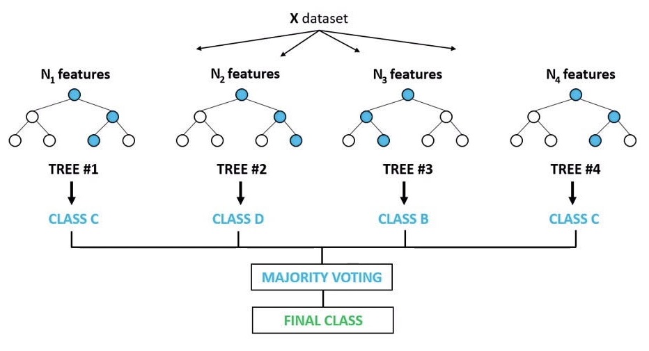
Random forest is model that combines multiple decision trees to make predictions. It averages across the individual tree predictions. Random forest can handle non-linear relationships, capture feature interactions, and effectively handle high-dimensional data. It provides robust predictions and reduces the risk of overfitting compared to individual decision trees.
Again, we set up our pipeline as follows:
Pipeline(steps=[('predictors',
                 ColumnSelector(columns=['genre.Crime', 'genre.Drama',
                                         'genre.Thriller', 'genre.Action',
                                         'genre.Horror',
                                         'genre.Science_Fiction', 'genre.Music',
                                         'genre.Reality', 'genre.Romance',
                                         'genre.Comedy', 'genre.Mystery',
                                         'genre.Documentary', 'genre.History',
                                         'genre.Teen',
                                         'genre.Health_&_Wellness',
                                         'genre.Lifestyle', 'genre.Culture',
                                         'genre.Blac...
                ('columntransform',
                 ColumnTransformer(remainder='passthrough',
                                   transformers=[('numericnaonehotencoder',
                                                  NumericNAOneHotEncoder(),
                                                  <sklearn.compose._column_transformer.make_column_selector object at 0x12d6d6610>),
                                                 ('onehotencoder',
                                                  OneHotEncoder(),
                                                  ['type', 'rating',
                                                   'country'])])),
                ('rf',
                 RandomForestRegressor(max_depth=10, min_samples_leaf=2,
                                       n_estimators=300))])
In a Jupyter environment, please rerun this cell to show the HTML representation or trust the notebook. Pipeline(steps=[('predictors',
ColumnSelector(columns=['genre.Crime', 'genre.Drama',
'genre.Thriller', 'genre.Action',
'genre.Horror',
'genre.Science_Fiction', 'genre.Music',
'genre.Reality', 'genre.Romance',
'genre.Comedy', 'genre.Mystery',
'genre.Documentary', 'genre.History',
'genre.Teen',
'genre.Health_&_Wellness',
'genre.Lifestyle', 'genre.Culture',
'genre.Blac...
('columntransform',
ColumnTransformer(remainder='passthrough',
transformers=[('numericnaonehotencoder',
NumericNAOneHotEncoder(),
<sklearn.compose._column_transformer.make_column_selector object at 0x12d6d6610>),
('onehotencoder',
OneHotEncoder(),
['type', 'rating',
'country'])])),
('rf',
RandomForestRegressor(max_depth=10, min_samples_leaf=2,
n_estimators=300))])ColumnSelector(columns=['genre.Crime', 'genre.Drama', 'genre.Thriller',
'genre.Action', 'genre.Horror', 'genre.Science_Fiction',
'genre.Music', 'genre.Reality', 'genre.Romance',
'genre.Comedy', 'genre.Mystery', 'genre.Documentary',
'genre.History', 'genre.Teen',
'genre.Health_&_Wellness', 'genre.Lifestyle',
'genre.Culture', 'genre.Black_Stories', 'genre.News',
'genre.Latino', 'genre.Adventure', 'genre.Anime',
'genre.Talk_Show', 'genre.Sketch_Comedy',
'genre.Family', 'genre.Kids', 'genre.Classics',
'genre.LGBTQ', 'genre.Adult_Animation', 'genre.Sitcom', ...])ColumnTransformer(remainder='passthrough',
transformers=[('numericnaonehotencoder',
NumericNAOneHotEncoder(),
<sklearn.compose._column_transformer.make_column_selector object at 0x12d6d6610>),
('onehotencoder', OneHotEncoder(),
['type', 'rating', 'country'])])<sklearn.compose._column_transformer.make_column_selector object at 0x12d6d6610>
NumericNAOneHotEncoder()
['type', 'rating', 'country']
OneHotEncoder()
['genre.Crime', 'genre.Drama', 'genre.Thriller', 'genre.Action', 'genre.Horror', 'genre.Science_Fiction', 'genre.Music', 'genre.Reality', 'genre.Romance', 'genre.Comedy', 'genre.Mystery', 'genre.Documentary', 'genre.History', 'genre.Teen', 'genre.Health_&_Wellness', 'genre.Lifestyle', 'genre.Culture', 'genre.Black_Stories', 'genre.News', 'genre.Latino', 'genre.Adventure', 'genre.Anime', 'genre.Talk_Show', 'genre.Sketch_Comedy', 'genre.Family', 'genre.Kids', 'genre.Classics', 'genre.LGBTQ', 'genre.Adult_Animation', 'genre.Sitcom', 'genre.Cooking_&_Food', 'genre.Sports', 'genre.Game_Shows', 'genre.International', 'genre.Cartoons', 'genre.Science_&_Technology', 'genre.Stand_Up', 'genre.Special_Interest', 'genre.Suspense', 'genre.TV_Shows', 'genre.Arts,_Entertainment,_and_Culture', 'genre.Variety', 'genre.Fantasy', 'genre.Young_Adult_Audience', 'genre.Animation', 'genre.Western', 'genre.Arthouse', 'genre.Unscripted', 'genre.Faith_and_Spirituality', 'genre.Military_and_War', 'genre.Independent_Movies', 'genre.British_TV_Shows', 'genre.Romantic_Movies', 'genre.Musical', 'genre.Comedies', 'genre.Classic_Movies', "genre.Kids'_TV", 'genre.Nature', 'genre.Cult', 'genre.Korean_TV_Shows', 'genre.Movies', 'genre.Biographical', 'genre.Superhero', 'genre.Coming_of_Age', 'genre.Anthology', 'genre.Buddy', 'genre.Parody', 'genre.Spy/Espionage', 'genre.Survival', 'genre.Soap_Opera_/_Melodrama', 'genre.Dance', 'genre.Medical', 'genre.Disaster']
passthrough
RandomForestRegressor(max_depth=10, min_samples_leaf=2, n_estimators=300)
Because a random forest contains many decision trees, you can tune both the hyperparameters of the forest and of the trees. We chose to again to tune n_neighbors and weights, and an additional hyperparameter n_estimators. This additional parameter controls the number of trees in the forest. Typically, more trees means a better model, and that is exactly what we found here, with n_estimators = 300. There seemed to be a drop off in the increase in performance around at 300 trees, so we didn’t search for values of n_estimators farther than that. The cross evaluation score of the random forest was a root mean squared error of 18.94.
The Decision Tree achieved a test rMSE of 19.03. This is almost a 3 point difference from the sample standard deviation of the scores (21.7), which means the beta regression predicts almost 3 rating points more accurately than guessing the mean, on average.
Here, you can input parameters for a Movie or TV Show and see each our models’ predictions for your show.